3D Single Shot

With CENOS platform it is possible to build and simulate full 3D induction hardening cases from imported CAD files. In this tutorial we will show you how to prepare and run an induction heating simulation from elsewhere created CAD file.

We will upload the pre-made CAD file into the CENOS platform, prepare it for meshing and mesh it while paying attention to the mesh quality and element count.

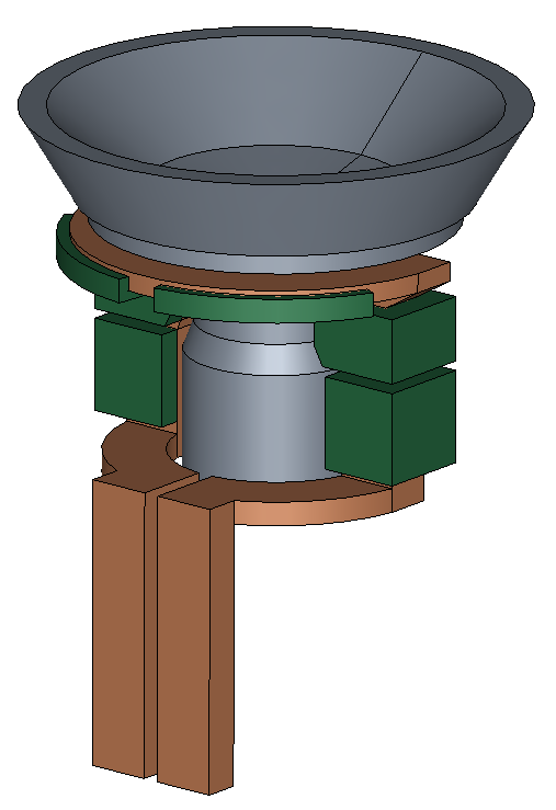
In the next pages a 3 s long induction hardening example of a rotating AISI 1020 workpiece at 5 kHz and 13 kA with custom shape inductor and FLUXTROL A yoke is presented.

Download the application files:

3D Single Shot.pdf

singleShotGeometry.zip

Simulation_tutorial_3D_singleShot.zip

IMPORTANT: If you feel like you want to create this geometry using the old GEOM module, click here to open this tutorial for GEOM module.

1. Open pre-processor

1.1 Choose pre-processing method and import CAD

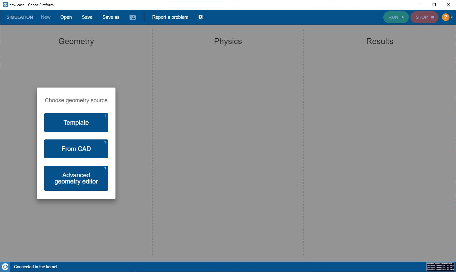
To manually create geometry and mesh, in CENOS home window click Advanced geometry editor.

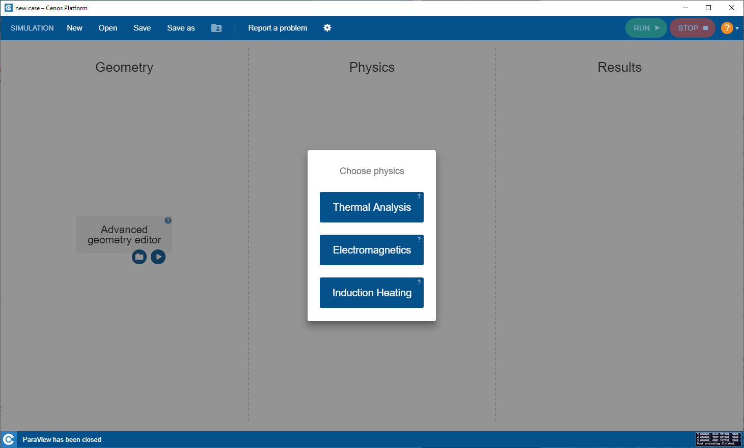
Click Induction Heating to select physics for simulation.

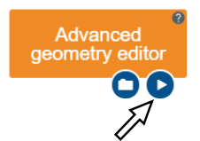
Click the Run icon to open salome.

Salome window with already selected Shaper module will open.

2. Create geometry and prepare it for meshing

2.1 Import geometry

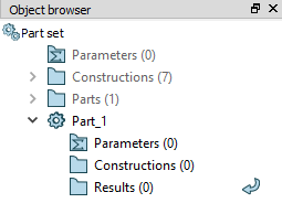
Create a new Part by clicking the New part () tool. A new part will be added to Object browser.

Click Import () and select the step file provided earlier.

To see the geometry, click Fit All ().

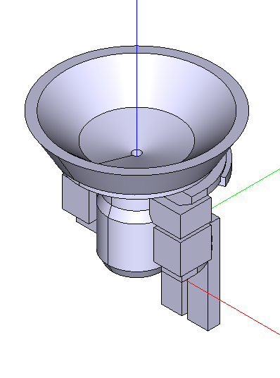
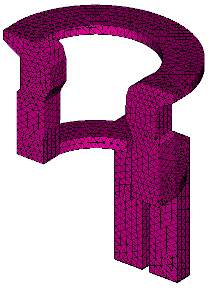
The imported geometry should look like this:

2.2 Create the air box

To correctly define inductor domain, one air box side must be in the same plane as the inductor terminals.

To achieve this, we will create a sketch on one of the inductor terminals. Click Sketch () tool and select one of the inductor terminals.

IMPORTANT: To rotate and move geometry around, toggle the Interaction style switch ().

Reposition the geometry by clicking +OZ () and disable Interaction style switch ().

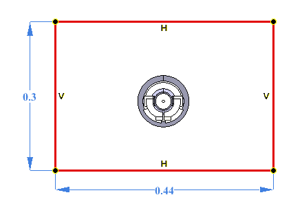
Select Rectangle () tool and draw a rectangle around the geometry. Click Length () tool and define the size of the rectangle (0.3m x 0.44m). Center it by eye:

Once completed, click Apply () and close the sketch.

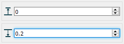
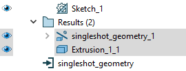
Now we need to extrude the rectangle we created. Click Extrusion () tool and select the rectangle. In the extrusion parameters enter 0.2m in the reverse direction:

2.3 Create Partition and Groups

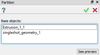
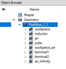
Click Partition () tool. From Object Browser select the imported geometry and created air box under Results and join them in one partition.

IMPORTANT: Partition and Groups are vital for simulation setup with CENOS, because mesh creation as well as physics and boundary condition definitions are based on the groups created in this part.

Click Group () tool and select the partition we just created (Partition_1_1). Choose the Shape Type, select one or more shapes from the screen, name the group and click Apply and continue ().

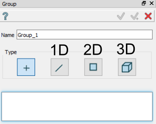
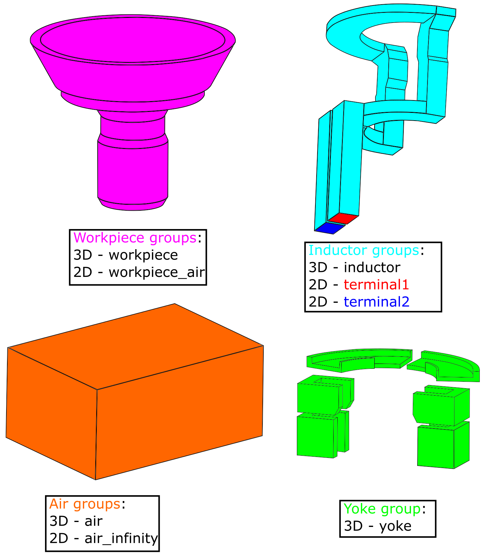
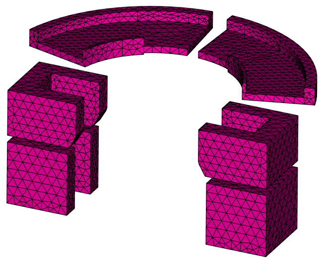
For this tutorial we will create four 3D groups for domains and four 2D groups for boundary conditions. The workpiece_air group includes full workpiece surface, while air_infinity includes all 6 sides of the air box, but without both terminals.

IMPORTANT: To select faces or volumes that are located within the Partition behind other objects and cannot be simply selected, you have to hide the partition and group in the object tab. Use the eye icon to toggle them.

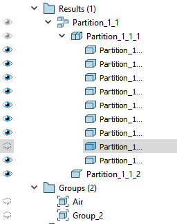
Detailed breakdown of these groups is as follows:

2.4 Export to GEOM

Finally we need to export the geometry created in Shaper to GEOM module. Do this by clicking Export to GEOM (). This will export the Partition and Groups to GEOM module, which is needed to proceed with mesh creation.

3. Create mesh and export it to CENOS

3.1 Switch to the Mesh module and create Mesh

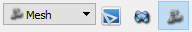
Switch to the Mesh module through Mesh icon or select it from the Salome module dropdown menu.

In Object Browser from Geometry dropdown menu select the previously created Partition_1_1 and click Create Mesh ().

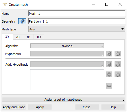
From the Assign a set of hypothesis dropdown menu select 3D: Automatic Tetrahedralization – leave the Max Length value default and click Apply and Close.

3.2 Create a sub-mesh for the workpiece

Right-click on Mesh_1 and click Create Sub-Mesh or select Create Sub-mesh () from the toolbar.

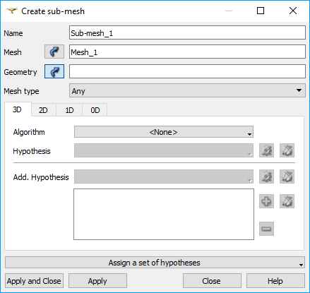
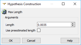
Select the workpiece group from the Partition_1_1 dropdown menu as Geometry. From the Assign a set of hypothesis dropdown menu select 3D: Automatic Tetrahedralization. In the Hypothesis Construction window enter 0.0035 for Max Length.

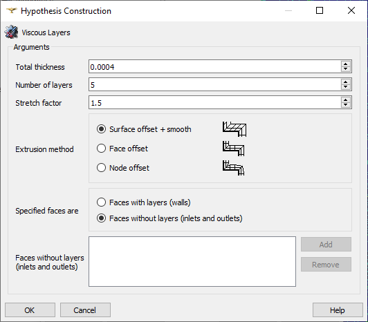
Resolve the skin layer on the surface of the workpiece by creating Viscous Layers. Under 3D algorithm section click the gear icon () next to Add. Hypotheses and select Viscous Layers.

Enter 0.0004 for Total thickness, 5 for Number of layers, 1.5 for Stretch factor and check the Faces without layers (inlets and outlets) box.

The 2D meshing algorithm will have to be changed to NETGEN 2D for it to mesh correctly. Under 2D change the algorithm and then click the gear icon next to Hypothesis and select Length From Edges.

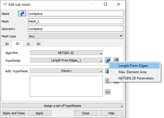
When all is set, click Apply and Close. Then right-click on just created sub-mesh and click Compute Sub-mesh to calculate and evaluate it.

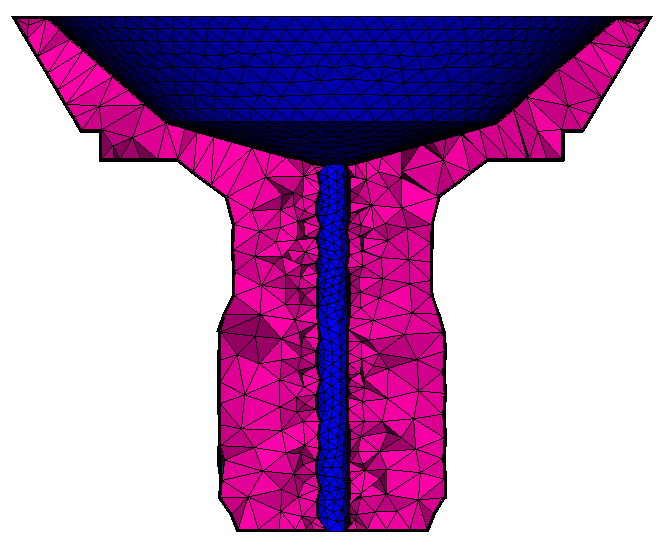
To see what the mesh looks like inside of an object such as workpiece, right-click on the previously calculated mesh in the VTK scene viewer window and select Clipping. In the Change Clipping window select Relative from the New dropdown menu, then select orientation of the clipping plane and click Apply and Close.

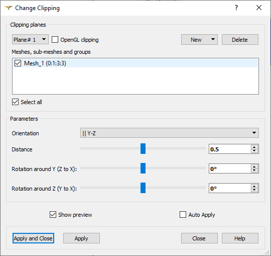
To return mesh to the unclipped state, enter the Change Clipping window and un-check the Mesh_1(0:1:2:3) box under Meshes, sub-meshes and groups.

3.3 Create a sub-mesh for the inductor

Create a sub-mesh and select the inductor group from the Partition_1_1 dropdown menu as Geometry. From the Assign a set of hypothesis dropdown menu choose 3D: Automatic Tetrahedralization and enter 0.003 for Max Length.

Resolve the skin layer on the surface of the workpiece by creating Viscous Layers. Under 3D algorithm section click the gear icon () next to Add. Hypotheses and select Viscous Layers.

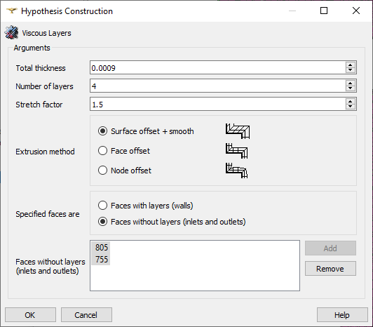
Select the groups terminal1 and terminal2 from the Partition_1_1 dropdown menu and click Add. Enter 0.0009 for Total thickness, 4 for Number of layers, 1.5 for Stretch factor and check the Faces without layers (inlets and outlets) box.

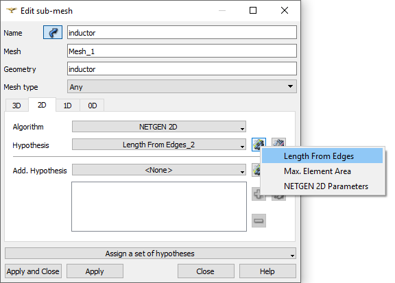
Again, the 2D meshing algorithm will have to be changed to NETGEN 2D. And the Hypothesis set to Length From Edges.

Calculate and evaluate the mesh.

3.4 Create a sub-mesh for the yoke

Create a sub-mesh and select the yoke group from the Partition_1_1 dropdown menu as Geometry. From the Assign a set of hypothesis dropdown menu choose 3D: Automatic Tetrahedralization and enter 0.003 for Max Length.

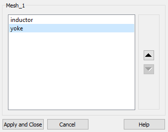
Before mesh calculation Salome will ask to set sub-mesh priorities, because the inductor and yoke geometries share common surfaces. Click Yes when the Warning window shows. Make sure that the inductor is above yoke, then click Apply and Close.

Calculate and evaluate the mesh.

3.5 Calculate and export the mesh to CENOS

Right-click on Mesh_1 and click Compute. Evaluate the final mesh and export it to CENOS. To do that, select Mesh_1 and select from the dropdown menu under Tools → Plugins → Mesh to CENOS to export your mesh to CENOS.

Before exporting the mesh to CENOS, the Select groups window will open and you will be asked to select the groups you want to export along with the mesh.

Select all the groups relevant for the physics setup, i.e. those who will be defined as domains or boundary conditions.

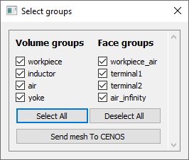
When selected, click Send mesh to CENOS.

4. Define physics and boundary conditions

4.1 Set the units and enter the physics setup

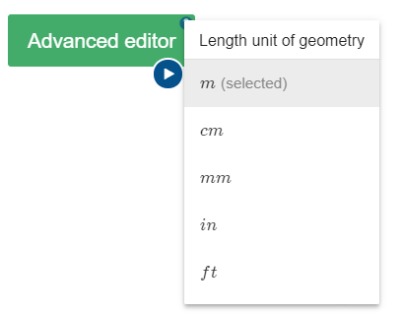
Wait until the mesh loads (see the spinner) and select the units by clicking on the gear icon next to the pre-processing block. In this tutorial we will select meters (m).

Click the gear icon under Induction Heating block to enter the physics setup.

4.2 Simulation control

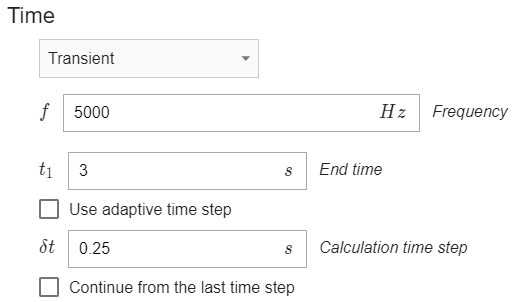
In the SIMULATION CONTROL window define the simulation as transient with 5 kHz frequency, 3 s End time and 0.25 s time step. For Computation algorithm choose Fast.

4.3 Workpiece definition

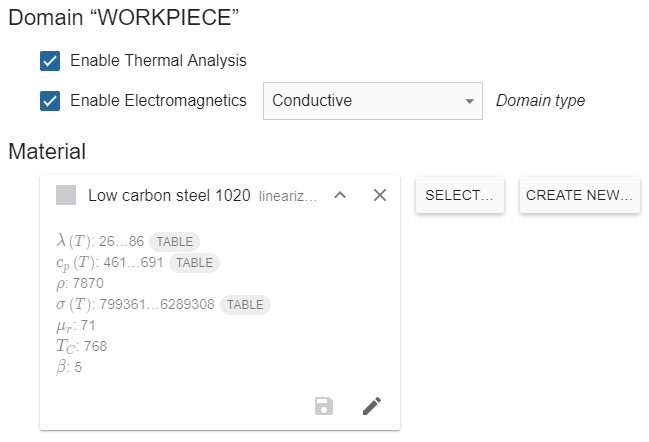
Select WORKPIECE from Domain bar. Leave Enable Thermal Analysis and Enable Electromagnetics boxes checked under Domain “WORKPIECE”. Choose Conductive as the domain type. For Material click SELECT… and choose Low carbon steel 1020 linearized (H=100000A/m), $t^{\circ}$ depend.

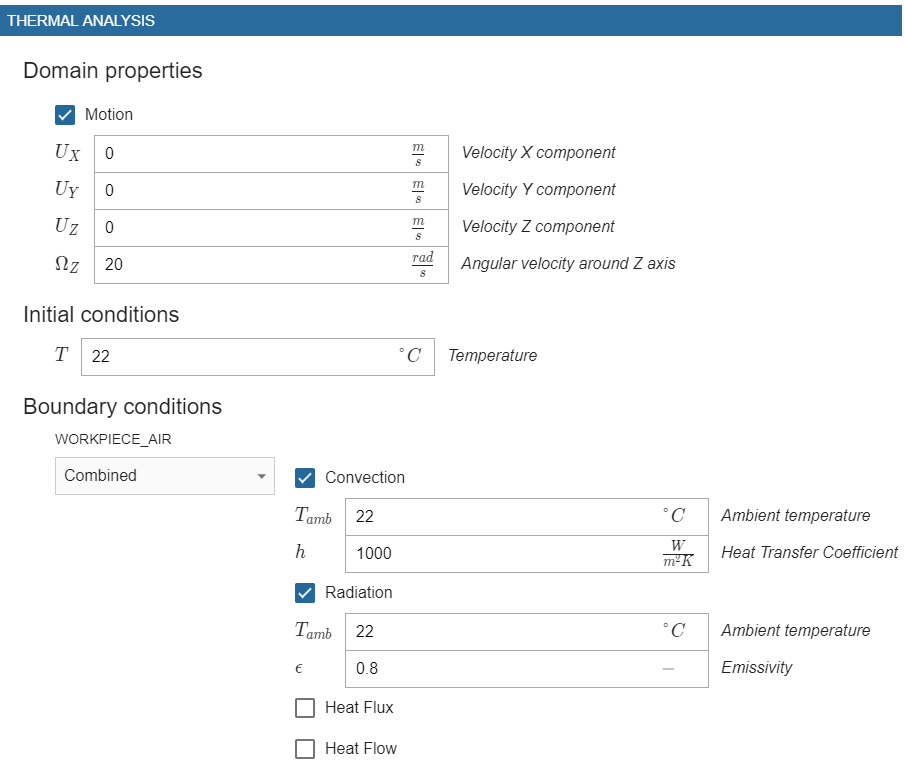
Under THERMAL ANALYSIS check the Motion box and enter 20 for Angular velocity around Z axis. For WORKPIECE_AIR choose Combined – check the Convection and Radiation boxes and enter 1000 for Heat Transfer Coefficient and 0.8 for Emissivity.

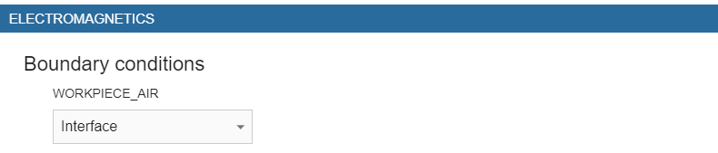
Under ELECTROMAGNETICS choose Interface for WORKPIECE_AIR.

4.4 Inductor definition

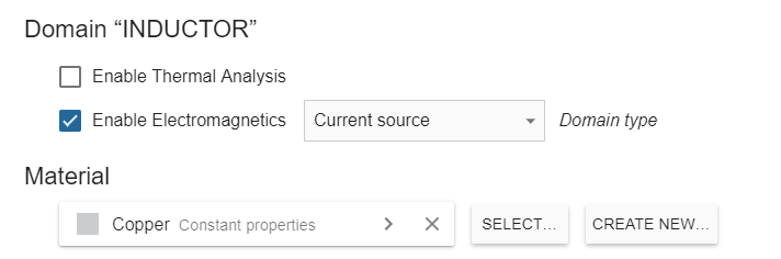
Switch to INDUCTOR in Domain bar. Disable Thermal analysis and select Current source as Domain type. For Material choose Copper Constant properties.

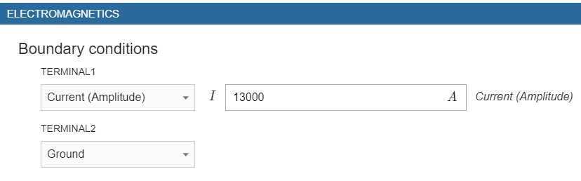
Under ELECTROMAGNETICS choose Current (Amplitude) for TERMINAL1, Ground for TERMINAL2 and enter 13000 A as Current (Amplitude).

4.5 Yoke definition

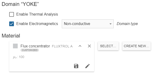
Switch to YOKE in Domain bar. For the yoke domain disable Thermal analysis and select Non-conductive as Domain type. For Material choose Flux concentrator FLUXTROL A. Disable B(H) curve and enter 100 for Magnetic permeability.

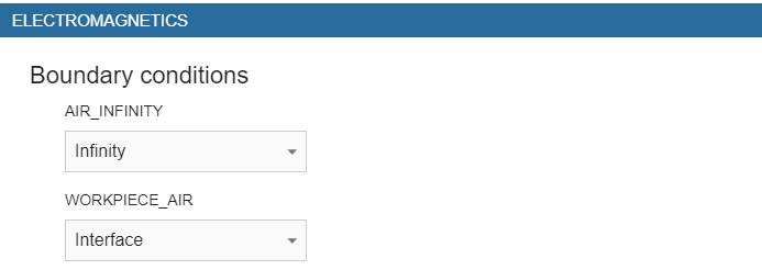
4.6 Air definition

For air domain disable Thermal analysis and select Non-conductive for Domain type. For Material choose Air.

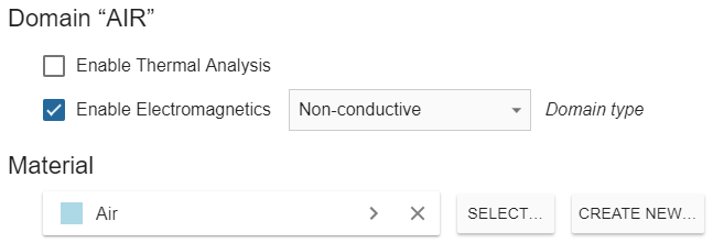
Under ELECTROMAGNETICS choose Infinity for AIR_INFINITY and Interface for WORKPIECE_AIR.

When everything is set, click RUN.

5. Evaluate results

When CENOS finishes calculation, a ParaView window with pre-set temperature result state will open and you will be able to see the temperature field distribution in the workpiece in the last time step.

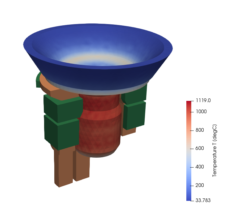
Results can be further manipulated by using ParaView filters - find out more in CENOS advanced post-processing article.

This concludes our 3D single shot induction heating simulation tutorial. For any recommendations or questions contact our support.