2D Scanning of Transmission Shaft
Induction heating of moving shafts and workpieces of any kind that are not regular in shape and size cannot be simply simulated using motion. CENOS platform incorporates scanning as a means of simulating movement of irregular workpiece through the inductor.
In this tutorial we will learn how to create and set up the simulation of a 30s long transmission shaft scanning at 7 kHz and 10 kA with two winding inductor.
Download the application files:
2D_Transmission_Shaft_Scanning.pdf
Simulation_tutorial_2D_scanning.zip
IMPORTANT: If you feel like you want to create this geometry using the old GEOM module, click here to open this tutorial for GEOM module.
1. Open pre-processor
1.1 Choose pre-processing method
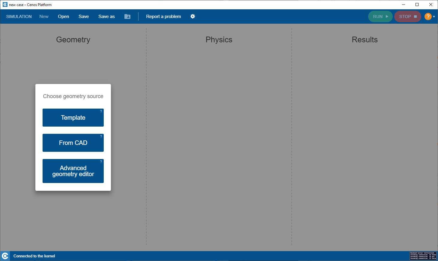
To manually create geometry and mesh, in CENOS home window click Advanced geometry editor.
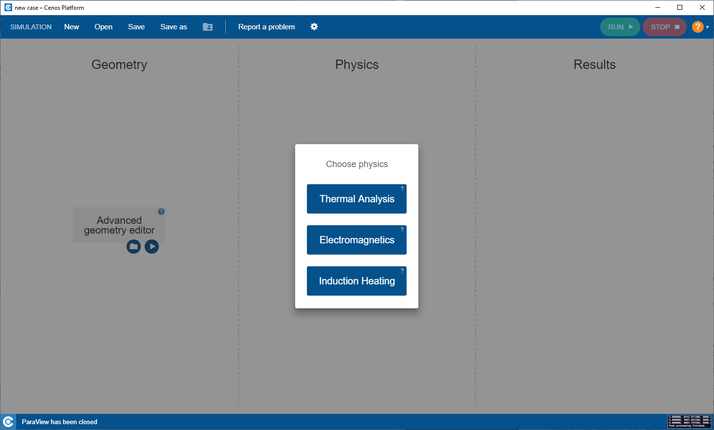
Click Induction Heating to select physics for simulation.
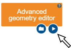
Click the Play icon to open Salome.
1.2 Load shaft geometry
In this tutorial we will not create the shaft geometry from scratch, but rather import it as Salome script.
IMPORTANT: To follow this tutorial, download the shaft geometry here. To learn how to create geometry from scratch, read stepped shaft or gear heating tutorials, or visit Salome documentation for more information about the Shaper module.
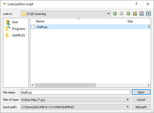
Click File → Load script....
In the Load python script window select and open previously downloaded shaft.py script file.
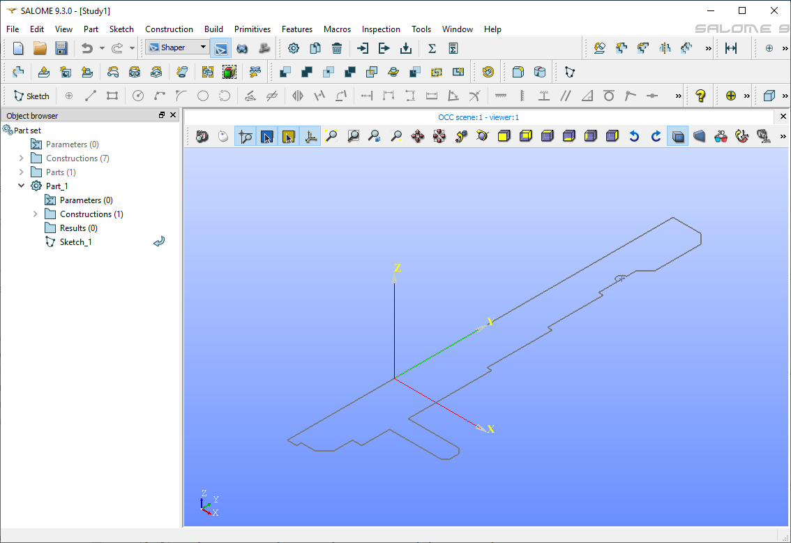
Once loaded you should see the geometry in the 3D viewer:
2. Create geometry and prepare it for meshing
Even though we imported the shaft geometry, we still need to create the inductor windings and air domain.
2.1 Create the inductor windings
In Object Browser right click on  and click Edit. By using Circle (
 ) tool create two circles, both 70 mm far from the Y axis and with 30 mm distance between them.
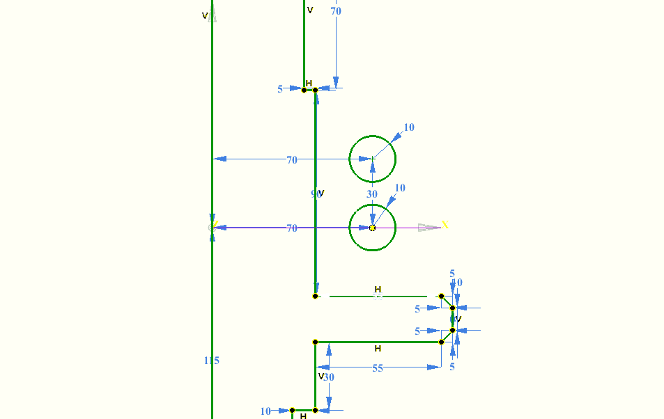
Use the constraints to set the dimensions:

If you cannot draw objects, you must disable camera control ( ).
).
2.2 Create the air box
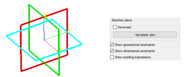
To create an air box, we first need to create a new sketch. Create a new Sketch by clicking the Sketch ( ) icon. Select the XY plane and click Set plane view
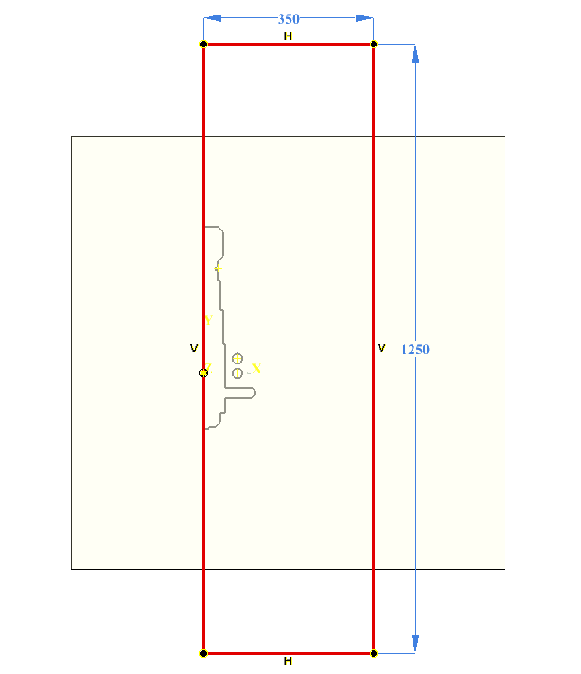
Create a rectangle (1250mm x 350mm) around the workpiece by clicking the Rectangle ( ) icon. Add a Coincidence (
 ) constraint between the symmetry axis edge (left side of the air box) and the origin point.
2.3 Create faces
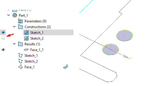
Create a face by clicking Face ( ) tool.
Select the inductor windings and the workpiece.
You might have to hide the air domain sketch to select the workpiece and inductor.
) tool.
Select the inductor windings and the workpiece.
You might have to hide the air domain sketch to select the workpiece and inductor.
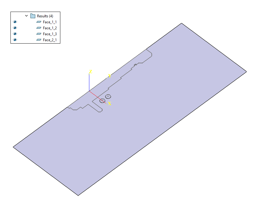
Now create the fourth air domain face and you should have all the faces as shown here:
2.4 Translate inductor windings
Click Translation ( ) tool. Select the middle option for the translation system, and select the two inductor faces we created. For DX and DZ enter 0. For DY enter scanning=0.
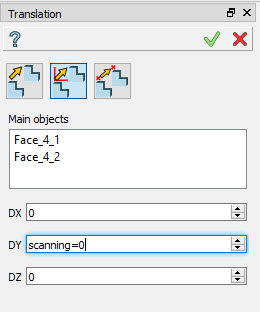
By entering "scanning=0", we automatically created a new parameter called "scanning" with a value of 0. You can use any name or value (within limits).
2.5 Create Partition and Groups
Click Partition ( ) tool, select previously created faces and join them in one partition.
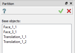
IMPORTANT: Partition and Groups are vital for simulation setup with CENOS, because mesh creation as well as physics and boundary condition definitions are based on groups created in this part.
Select Group ( ) tool and choose the Shape Type. Select one or more shapes from the screen, name the group and click the Apply and continue (
 ).
).
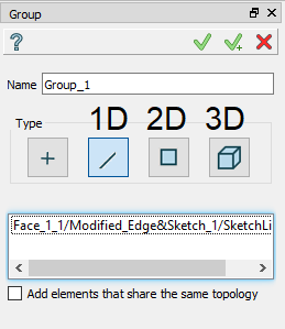
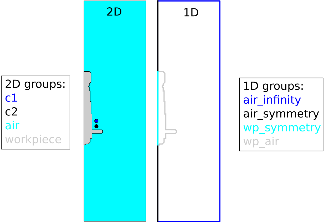
For this tutorial we will create four 2D groups for domains and four 1D groups for boundary conditions. When creating groups, select only those objects relevant for the specific group.
A detailed breakdown of these groups is as follows:
2.7 Export to GEOM
Finally we need to export the geometry created in Shaper to GEOM module. Do this by clicking Export to GEOM ( ). This will export the Partition and Groups to GEOM module, which is needed to proceed with mesh creation.
3. Create mesh and export it to CENOS
3.1 Switch to Mesh module and create Mesh
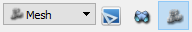
Switch to the Mesh module through Mesh icon or select it from the Salome module dropdown menu.
In Object Browser from Geometry dropdown menu select the previously created Partition_1_1 and click Create Mesh ( ).
).
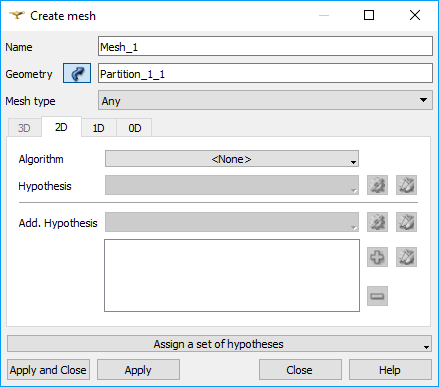
From the Assign a set of hypothesis dropdown menu select 2D: Automatic Triangulation - leave the Max Length value default and click Apply and Close.
3.2 Create a sub-mesh for the workpiece
Right-click on Mesh_1 and click Create Sub-Mesh or select Create Sub-mesh ( ) from the toolbar.
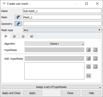
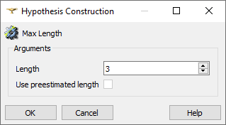
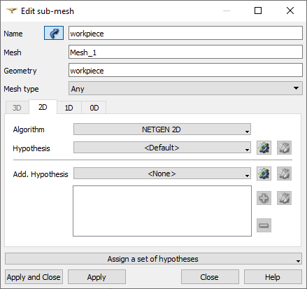
Choose workpiece group from the Partition_1_1 dropdown menu as Geometry. From the Assign a set of hypothesis dropdown menu choose 2D: Automatic Triangulation. In the Hypothesis Construction window enter 3 for Max Length and change the 2D algorithm from Triangle: Mefisto to NETGEN 2D.
Resolve the skin layer on the surface of the workpiece by creating Viscous Layers. Click the gear icon ( ) next to Add. Hypotheses and select Viscous Layers 2D.
Select the group wp_air from the Partition_1_1 dropdown menu and click Add. Enter 0.4 for Total thickness, 5 for Number of layers, 1.25 for Stretch factor and check the Edges with layers (walls) box.
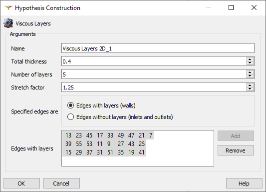
When all is set, click Apply and Close.
3.3 Create a sub-mesh for the inductor
Create a sub-mesh and select c1 and c2 groups from the Partition_1_1 dropdown menu as Geometry. From the Assign a set of hypothesis dropdown menu choose 2D: Automatic Triangulation and enter 3 for Max Length.
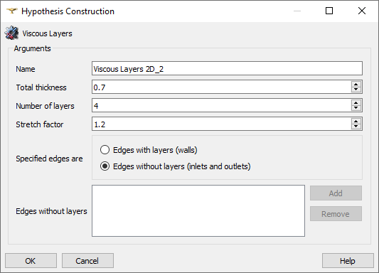
Resolve the skin layer on the surface of the workpiece by creating Viscous Layers. Click the gear icon () next to Add. Hypotheses and select Viscous Layers 2D.
Enter 0.7 for Total thickness, 4 for Number of layers, 1.2 for Stretch factor and check the Edges without layers (inlets and outlets) box.
IMPORTANT: If you create a sub-mesh from multiple groups, Salome will auto-group them and create a new group, in this case named Auto_group_for_Sub-mesh_2.
3.4 Calculate and export mesh to CENOS
Right-click on Mesh_1 and click Compute. Evaluate the final mesh and export it to CENOS. To do that, select Mesh to CENOS from the dropdown menu under Tools → Plugins → Mesh to CENOS to export your mesh to CENOS.
Before exporting mesh to CENOS, the Select groups window will open and you will be asked to select the groups you want to export along with the mesh.
Select all groups relevant for the physics setup, i.e. those who will be defined as domains or boundary conditions. We will select all groups except Auto_group_for_Sub-mesh_2.
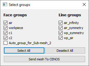
When selected, click Send mesh to CENOS.
4. Define physics and boundary conditions
4.1 Set units and enter physics setup
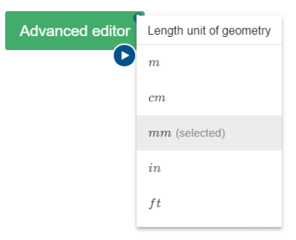
Wait until the mesh loads (see the spinner) and select the units by clicking on the gear icon next to the pre-processing block. In this tutorial we will select millimeters (mm).
Click the gear icon under Induction Heating block to enter the physics setup.

4.2 Simulation control
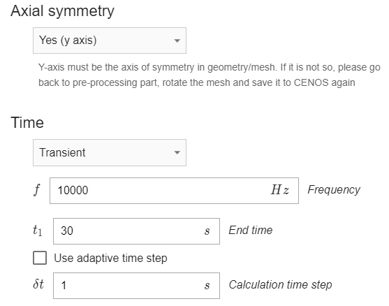
In SIMULATION CONTROL window define the simulation as axial symmetric and transient with 10 kHz frequency, 30 s End time and 1 s time step.
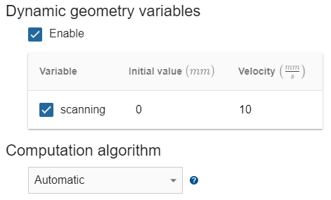
Check the Dynamic geometry variables check box. Leave the Initial value 0 mm and enter 10 for Velocity. For Computation algorithm leave Automatic.
4.3 Workpiece definition
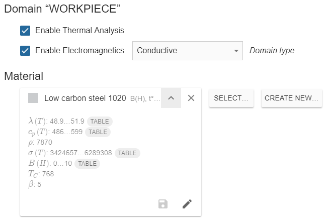
Switch to WORKPIECE in Domain bar. Leave Enable Thermal Analysis and Enable Electromagnetics boxes checked under the Domain “WORKPIECE”. Choose Conductive as the domain type. For Material click SELECT… and choose Low carbon steel 1020 B(H), %% t^{\circ} %% depend.
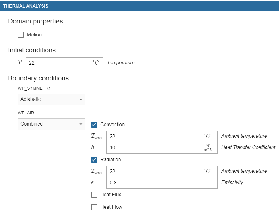
Under THERMAL ANALYSIS for boundary conditions choose Combined for WP_AIR – check the Convection and Radiation boxes and enter 10 for Heat Transfer Coefficient and 0.8 for Emissivity. Choose Adiabatic for WP_SYMMETRY.
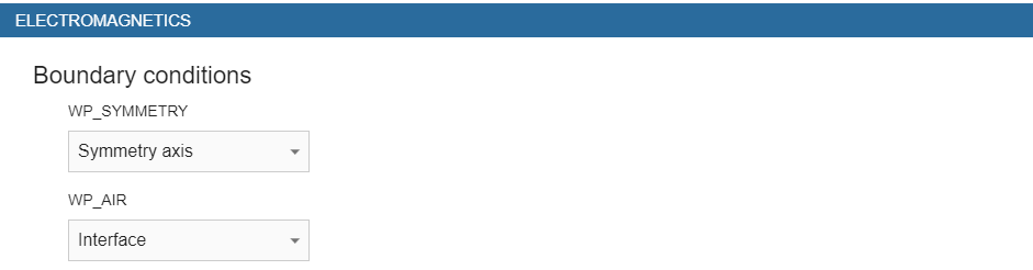
Under ELECTROMAGNETICS choose Interface for WP_AIR and Symmetry axis for WP_SYMMETRY.
4.4 Coil definition
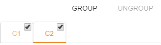
We created 2 different domains for each winding in order to define the current for each of them. To save time, it is possible to group these domains and define them all through one Setup window. To do that, select all winding domains and click GROUP.
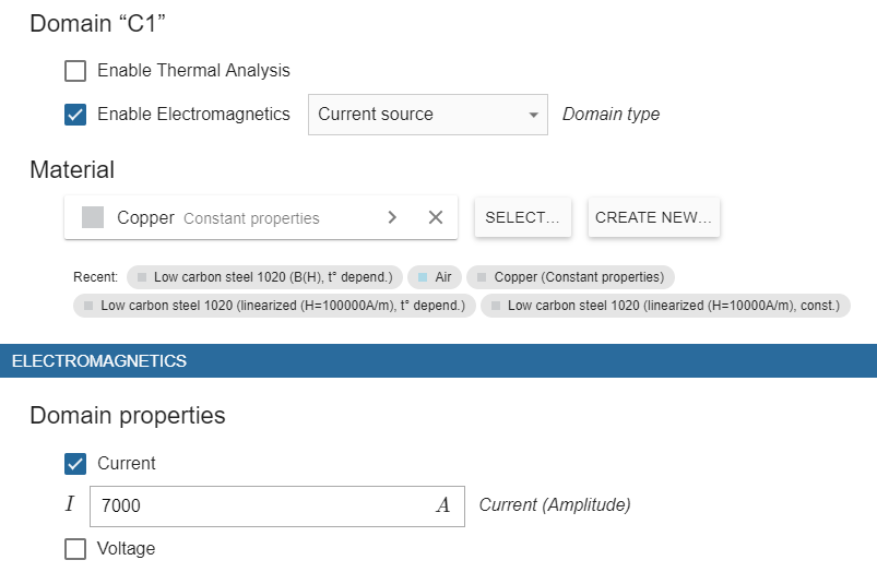
Disable Thermal analysis and select Current source for Domain type. For Material choose Copper Constant properties and enter 7000 A for Current (Amplitude).
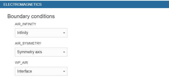
4.5 Air definition
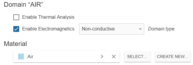
Switch to AIR in Domain bar. Disable Thermal analysis and select Non-conductive as Domain type. For Material choose Air.
Under ELECTROMAGNETICS choose Infinity for AIR_INFINITY, Symmetry axis for AIR_SYMMETRY and Interface for WP_AIR.
When everything is set, click RUN.
5. Evaluate results
When CENOS finishes calculation, ParaView window with pre-set temperature result state will open automatically and you will be able to see the temperature field distribution in workpiece in the last time step as well as a 3D revolution of the results to give you better visual interpretation.
Results can be further manipulated by using ParaView filters - find out more in CENOS advanced post-processing article.
This concludes our Transmission Shaft Scanning tutorial. For any recommendations or questions contact our support.